DetectoRS — A Comprehensive Review
Summary
A detailed breakdown of a new paper from Google Research and Johns Hopkins University — DetectoRS: Detecting Objects using Recursive Feature Pyramids and Switchable Atrous Convolutions.
Table of Contents
There has been extensive research going on in finding novel techniques, algorithms, and new end-to-end trainable pipelines for Object Detection and Image Segmentation tasks in the field of Computer Vision.
Year by year, different research institutes/organizations come up with some new ideas to tackle the pertaining problems of these tasks with robust and real-time solutions.
Given the premise, 2020 is being one of the most exciting years for the field of Computer Vision and Deep Learning.
In June 2020, Google Research Team with Johns Hopkins University came up with an exciting new architecture design of Feature Pyramid Networks and modulation of existing convolutional operation chains in the paper DetectoRS: Detecting Objects using Recursive Feature Pyramids and Switchable Atrous Convolutions[1] that can be directly leveraged into the present neural network backbones such as ResNets, ResNeXts, etc.
This paper claimed to have a state-of-the-art performance on COCO Object Detection/Image Segmentation Dataset with an mAP of 54.7% and mask AP of 47.1% respectively.
In this article, we will go through the critical baselines mentioned in the paper. Let’s jump right in.
1. Introduction
- Recently, the coupling of thinking and looking twice mechanism in state-of-the-art two-stage object detectors has proved to give promising results in image segmentation and object detection tasks.
- Object detectors such as Faster RCNN first detects the object proposals based on the foreground-background classification, which are then used to extract rich semantic features for further classification/detection tasks in later stages.
- Following thinking and looking twice regime, Cascade RCNN is designed to refine these obtained proposals from one stage and enrich these proposals with their multi-stage design, as shown in Fig. 1. As we continue to go deep inside the network, subsequent head classifiers/detectors are trained on more enhanced object features.
- Inspired by this, the authors introduced a novel approach to leverage this mechanism directly in the network backbone.
- They consider the Hybrid Task Cascade network as their baseline architecture for comparison studies.
HTC is a version up of Cascade Faster-RCNN, but have an extra module for image segmentation mask. You can visualize it from Fig. 2.
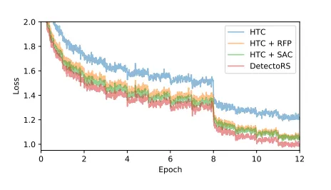
The proposition of Switchable Atrous Convolutions and Recursive Feature Pyramid Networks at the macro(Neck) and micro(Backbone Convolutions) levels of the network respectively significantly improved the state-of-the-art network HTC with almost the same inference time[1].
| Method | Backbone | AP box | AP mask | FPS |
|---|---|---|---|---|
| HTC | ResNet-50 | 43.6 | 38.5 | 4.3 |
| DetectoRS | ResNet-50 | 51.3 | 44.4 | 3.9 |
Table. 1 Inference and mAP number comparison between HTC and DetectoRS.
2. Proposed Workflow
- The authors were more focused on the present refinements of the convolutions operations and Feature Pyramid Networks to incorporate the stated regime in current models.
- Recursive Feature Pyramid Networks and Switchable Atrous Convolution are two significant findings mentioned in the paper.
- At the macro level, they introduced a new version of Feature Pyramids, by connecting the top-down level path predictions as a feedback loop to the bottom-up path, as shown in Fig. 3.
![Fig.3 Feedback prediction feature maps to bottom-up layers(Source: [1]).](/images/reads/detectors/05.webp)
Unrolling the recursive structure to a sequential implementation, we obtain a backbone for an object detector that looks at the images twice or more. Similar to the cascaded detector heads in Cascade R-CNN trained with more selective examples, our RFP recursively enhances FPN to generate increasingly powerful representations[1].
- At the micro-level, they propose SAC(Switchable Atrous Convolutions), which takes feature maps as input and convolves with different atrous rates based on the global context information and combines the output using the switch functions as shown in Fig. 4.
![Fig. 4 Switch function for different atrous rates(Source: [1]).](/images/reads/detectors/06.webp)
The switch functions are spatially dependent, i.e., each location of the feature map might have different switches to control the outputs of SAC. To use SAC in the detector, we convert all the standard 3x3 convolutional layers in the bottom-up backbone to SAC, which improves the detector performance by a large margin[1].
Recursive Feature Pyramid Networks
- Let’s revisit the structure of the basics of Feature Pyramid Networks. Here, B(i) denotes the bottom-up downsampling layer chains. F(i) is the top-down FPN operation.
- B(i) takes x(i-1) high resolution feature map. and convert it into low-resolution alternative x(i), as shown in Fig. 5.
- Also, prediction feature maps f(i) are passed to the prediction head for further classification and regression. Top-down layer F(i) takes input the bottom-up feature map x(i) and low-resolution alternative f(i+1). All f(i)s are the set of prediction feature maps. It can be generalized by the equation as:-
Source: [1]
- Now, in Recursive Feature Pyramids, as the name depicts, each FPN layer is stacked T times. Output prediction maps f(i) in Fig 5. are used as feedback loops in the bottom-up downsampling layer chains B(i)(The feedback loop structure can be visualized from Fig. 3). Let’s magnify that image to see how the unrolling happens in RFP.
- The above figure shows the two-stage(t = 2) unrolling of the Recursive Feature Pyramids. Blue shaded region is the same backbone(or different backbone. We will see this in the implementation details section) used for the first stage bottom-up FPN operation.
- Before passing the prediction feature maps f(i) to the backbone again, they are passed through the ASPP Module as shown. This is called transformation R(i) on feature map f(i). We can generalize this network design for different values of stacking stage t with the below-given equation.
- Here, t ∈[2, 3, …, T] is the number of unrolling operation to be done. By default, T = 2.
- There are two main pre-requisites or transformation parts used in RFP viz. ASPP(Atrous Spatial Pyramid Pooling) and Fusion Module.
ASPP(or Atrous Spatial Pyramid Pooling) module does the same thing to increase the receptive field of the network, but instead of using standard convolutions of different kernel sizes, dilated convolutions with different atrous rates are used. Its implementation in RFP can be visualized from the below-given figure.
- ASPP module output features are directly passed to the first residual block of every layer of the ResNet. It takes both x(i) and R(f(i)) as an input to the residual block. Visualization is given below.
The weight of RFP 1x1 convolutional layer is initialized with 0 to make sure it does not have any real effect when pretrained weights are used for training downstream tasks[1]. RFP Features are only applied on t = [2, …, T] stages. First stage is a default FPN operation.
- The different combinations of feature fusion and attention layer techniques have performed very well in the deep networks to detect the varied objects at different scales with a decent confidence score.
- The authors, to further improvise the information of the maps added Fusion Module that uses the top-down FPN operation feature maps(f(i)s as shown in Fig. 6) from different stages of FPN and combines them together with an implicit attention gate in their design. Visualization is given below.
Feature fusion module is only applied at the unrolled steps from t=[2, …, T]. Module takes the present newly obtained top-down operation feature map f(i+1) at an unrolled step t + 1 and f(i) at t respectively. Sigmoid function generates an intermediary attention map for the present features and are used in the aggregation of both the inputs. Output of this module is the more focused feature map f(i+1) at unrolled step t + 1
What is the logic behind a cascaded FPN(or Recursive Feature Pyramid) structure?
- We all know that as we go deep in the network, semantic information about the objects increases and the system tries to learn well while keeping a global context in mind. Also, earlier layers are crucial to learning low-level information such as edges, textures giving proper discriminative features.
- Cascading and connecting the output maps to the backbone structures(Fig. 8) further at the unrolled stages can help to capture the missed information about the objects by keeping in mind the receptive field and context using ASPP, and remove the unwanted activated pixels values with the help of implicit attention layer in Fusion Stage.
This is the official RFP code on their repository. You can visit the code structure for getting implementation insights.
Switchable Atrous Convolutions
- Atrous(or Dilated) Convolutions are the operation that increases the field of view without any additional computations.
- The receptive field is an essential concept in Convolutional Neural Networks. A large kernel size can increase the output context information of the feature map with the cost of increasing the computations.
Atrous convolution with atrous rate r introduces r − 1 zero between consecutive filter values, equivalently enlarging the kernel size of a k × k filter to knew = k + (k − 1)(r − 1) without increasing the number of parameters or the amount of computation[1].
- As stated, a 3x3 convolutional kernel can give the same receptive as 5x5 with fixed computational multiplications by keeping atrous rate r = 2.
- By using dilated convolutions with higher atrous rates can sometimes miss capturing the local information of the objects at smaller scales.
- Conditional convolutions such as Selective Kernel Networks, Dynamic Convolutions, etc. are some of the present and well-known implementations of the dynamic, receptive field adjustment based on the scales and context of the objects. But these implementations are somewhat ineffective while using the pretrained network architectures.
- So, the authors introduced a new concept of the conditional convolutions that can be used as a to-go choice for pretrained backbone networks.
- They also introduced a very intuitive switch and context mechanism in the convolution overview(shown in Fig. 11) to generate effective results.
- All 3x3 convolution operations in the residual blocks of the ResNet are changed to dilated convolutions with two different atrous rates, as shown in Fig. 11.
Both the convolution operations shares the same weight w.
The above equation shows the switching mechanism between two convolution operations. Both share the same weights with a different trainable δw(Source: [1]).
- S(x) is a switch function that consists of an Average Pooling Layer of 5x5 kernel followed by a 1x1 convolution block. This switch can gather some statistics of the feature map using pooling layers, which can be further used to detect objects at different scales.
A value obtained from the patch of an average pooling operation is a decision-maker to increase the field of view or not. If the pooling operation does not activate the feature map pixels then a convolution operation with a large field of view(or dilated convolution) might be more canonical to obtain better statistics of the object if present.
- The global context mechanism is also added before and after each of the 3x3 blocks. These are lightweight 1x1 convolution kernels and a global average pooling layer. They state that using global information is more efficient for a switch function S(x) to stabilize the switching between two convolution operations.
Object detectors usually use pretrained checkpoints to initialize the weights. However, for a SAC layer converted from a standard convolutional layer, the weight for the larger atrous rate is missing. Since objects at different scales can be roughly detected by the same weight with different atrous rates, it is natural to initialize the missing weights with those in the pretrained model[1].
∇w is compensation parameter for the atrous convolutions and is initialized to zero. This weight differences are the small precision values for the original pretrained weights for atrous convolutions.
You can get a proper flow of SAC from this code.
The Python behind this figure
3. Results
- The authors took the Hybrid Task Cascade framework as a baseline and added the above two novel designs to obtain DetectoRS.
- Backbone architectures considered were the ResNet family variant such as ResNet-50 and ResNeXt-101–32x4d. Also, all the 3x3 convolution operations were replaced by Deformable Convolutions.
- The offset values of the DCN and weight difference ∇w were initialized to 0.
- The weights and biases of the Pre and Post Context 1x1 convolutional kernels were initialized to zeros and ones, respectively.
| AP | AP50 | AP75 | APS | APM | APL | |
|---|---|---|---|---|---|---|
| Baseline HTC | 42.0 | 60.8 | 45.5 | 23.7 | 45.5 | 56.4 |
| RFP | 46.2 | 65.1 | 50.2 | 27.9 | 50.3 | 60.3 |
| RFP + sharing | 45.4 | 64.1 | 49.4 | 26.5 | 49.0 | 60.0 |
| RFP - aspp | 45.7 | 64.2 | 49.6 | 26.7 | 49.3 | 60.5 |
| RFP - fusion | 45.9 | 64.7 | 50.0 | 27.0 | 50.1 | 60.1 |
| RFP + 3X | 47.5 | 66.3 | 51.8 | 29.0 | 51.6 | 61.9 |
| SAC | 46.3 | 65.8 | 50.2 | 27.8 | 50.6 | 62.4 |
| SAC - DCN | 45.3 | 65.0 | 49.3 | 27.5 | 48.7 | 60.6 |
| SAC - DCN - global | 44.3 | 63.7 | 48.2 | 25.7 | 48.0 | 59.6 |
| SAC - DCN - locking | 44.7 | 64.4 | 48.7 | 26.0 | 48.7 | 59.0 |
| SAC - DCN + DS | 45.1 | 64.6 | 49.0 | 26.3 | 49.3 | 60.1 |
Table. 1 Ablation Study for different variations of the parameters
- We can see from the above table that different backbone weights(weights B(t=1) ≠weights B(t=2)) and three-stage unrolling(t=3) gave the best results.
- Also, by using the locking mechanism of the weights between two atrous convolutions gave better results rather than just using ∇w for training.
| Method | Backbone | TTA | AP bbox | AP50 | AP75 | APS | APM | APL |
|---|---|---|---|---|---|---|---|---|
| YOLOv3 | DarkNet-53 | 33.0 | 57.9 | 34.4 | 18.3 | 25.4 | 41.9 | |
| RetinaNet | ResNeXt-101 | 40.8 | 61.1 | 44.1 | 24.1 | 44.2 | 51.2 | |
| RefineDet | ResNet-101 | ✓ | 41.8 | 62.9 | 45.7 | 25.6 | 45.1 | 54.1 |
| CornerNet | Hourglass-104 | ✓ | 42.1 | 57.8 | 45.3 | 20.8 | 44.8 | 56.7 |
| ExtremeNet | Hourglass-104 | ✓ | 43.7 | 60.5 | 47.0 | 24.1 | 46.9 | 57.6 |
| FSAF | ResNeXt-101 | ✓ | 44.6 | 65.2 | 48.6 | 29.7 | 47.1 | 54.6 |
| FCOS | ResNeXt-101 | 44.7 | 64.1 | 48.4 | 27.6 | 47.5 | 55.6 | |
| CenterNet | Hourglass-104 | ✓ | 45.1 | 63.9 | 49.3 | 26.6 | 47.1 | 57.7 |
| NAS-FPN | AmoebaNet | 48.3 | - | - | - | - | - | |
| SEPC | ResNeXt-101 | 50.1 | 69.8 | 54.3 | 31.3 | 53.3 | 63.7 | |
| SpineNet | SpineNet-190 | 52.1 | 71.8 | 56.5 | 35.4 | 55.0 | 63.6 | |
| EfficientDet-D7 | EfficientNet-B6 | 52.6 | 71.6 | 56.9 | - | - | - | |
| Mask R-CNN | ResNet-101 | 39.8 | 62.3 | 43.4 | 22.1 | 43.2 | 51.2 | |
| Cascade R-CNN | ResNet-101 | 42.8 | 62.1 | 46.3 | 23.7 | 45.5 | 55.2 | |
| Libra R-CNN | ResNeXt-101 | 43.0 | 64.0 | 47.0 | 25.3 | 45.6 | 54.6 | |
| DCN-v2 | ResNet-101 | ✓ | 46.0 | 67.9 | 50.8 | 27.8 | 49.1 | 59.5 |
| PANet | ResNeXt-101 | 47.4 | 67.2 | 51.8 | 30.1 | 51.7 | 60.0 | |
| SINPER | ResNet-101 | ✓ | 47.6 | 68.5 | 53.4 | 30.9 | 50.6 | 60.7 |
| SNIP | Model Ensemble | ✓ | 48.3 | 69.7 | 53.7 | 31.4 | 51.6 | 60.7 |
| TridentNet | ResNet-101 | ✓ | 48.4 | 69.7 | 53.5 | 31.8 | 51.3 | 60.3 |
| Cascade Mask R-CNN | ResNeXt-152 | ✓ | 50.2 | 68.2 | 54.9 | 31.9 | 52.9 | 63.5 |
| TSD | SENet154 | ✓ | 51.2 | 71.9 | 56.0 | 33.8 | 54.8 | 64.2 |
| MegDet | Model Ensemble | ✓ | 52.5 | - | - | - | - | - |
| CBNet | ResNeXt-152 | ✓ | 53.3 | 71.9 | 58.5 | 35.5 | 55.8 | 66.7 |
| HTC | ResNet-50 | 43.6 | 62.6 | 47.4 | 24.8 | 46.0 | 55.9 | |
| HTC | ResNeXt-101-32x4d | 46.4 | 65.8 | 50.5 | 26.8 | 49.4 | 59.6 | |
| HTC | ResNeXt-101-64x4d | 47.2 | 66.5 | 51.4 | 27.7 | 50.1 | 60.3 | |
| HTC + DCN + mstrain | ResNeXt-101-64x4d | 50.8 | 70.3 | 55.2 | 31.1 | 54.1 | 64.8 | |
| DetectoRS | ResNet-50 | 51.3 | 70.1 | 55.8 | 31.7 | 54.6 | 64.8 | |
| DetectoRS | ResNet-50 | ✓ | 53.0 | 72.2 | 57.8 | 35.9 | 55.6 | 64.6 |
| DetectoRS | ResNeXt-101-32x4d | 53.3 | 71.6 | 58.5 | 33.9 | 56.5 | 66.9 | |
| DetectoRS | ResNeXt-101-32x4d | ✓ | 54.7 | 73.5 | 60.1 | 37.4 | 57.3 | 66.4 |
Table 2. DetectoRS comparisons with different object detectors on COCO-test dev.
Official Github Code: [github]
4. Conclusion
- The authors introduced the two novel techniques, viz. Switchable Atrous Convolutions and Recursive Feature Pyramid Networks.
- They followed the regime of thinking and looking twice inspired from the network designs of Cascade RCNN, Hybrid Task Cascade, etc. by connecting the feedback loop in the unrolled cascade FPNs.
- By leveraging the two novel methods with HTC as a baseline, it outperformed every present model in object detection, image, and panoptic segmentation with COCO mAP of 54.7%.
Different ablation studies conducted by the authors to find the legitness of the model spaces are skipped in this article. You can get to know about the different permutations of the network parameters from the paper. Image and Panoptic Segmentation are also not mentioned in this article as they were not intersecting with the scope of this article.
I hope you found the content meaningful. If you want to stay updated with the latest research in AI, please follow us at VisionWizard.
5. References
[1] DetectoRS: Detecting Objects with Recursive Feature Pyramid and Switchable Atrous Convolution
6. Connections
What this read builds on, and what builds on it. Hover a box for a preview.
Related
- Read · this builds on it
- Read · same topic: object detection
- Read · same topic: object detection
- Read · same topic: object detection
- Project · same topic: object detection
- Project · same topic: object detection
Go deeper
-
Start withRead
-
You are hereDetectoRS — A Comprehensive ReviewRead