YOLOv4 — Version 4: Final Verdict
Summary
An Introductory Guide on the Fundamentals and Algorithmic Flows of YOLOv4 Object Detector
Table of Contents
- 1. Finalizing Bag of Freebies attributes2
- 2. Finalizing Bag of Specials attributes2
- 3. Effect of BoF + BoS on Training MiniBatch Size2
- 4. Results of Backbone + Neck + Head2
- 5. Comparison of mAP and FPS with different Object Detectors2
- 6. References2
- 7. Connections2
Welcome to the final part of YOLOv4¹ mini-series.
YOLOv4 — Version 0: Introduction
YOLOv4 — Version 1: Bag of Freebies
YOLOv4 — Version 2: Bag of Specials
YOLOv4 — Version 3: Proposed Workflow
YOLOv4 — Version 4: Final Verdict
I hope we were able to do a thorough walk through of all nuts and bolts of this amazing research.
This article’s main focus is on analytical results rather than any informative explanations. One last ride, let’s begin the finale.
This article will state the analytical comparisons between yolov4 and other object detectors.
1. Finalizing Bag of Freebies attributes
- As discussed in the introduction of this series, many candidates were taken into consideration and were finalized to a small subset of them. We can analyze from the given tables below, how it affects the accuracy of the model.
- Results given below in the form of tables are self-explanatory. The number’s speak for itself.
- S: Eliminate grid sensitivity the equation bx = σ(tx) + cx, by = σ(ty) + cy, where cx and cy are always whole numbers, is used in YOLOv3 for evaluating the object coordinates, therefore, extremely high tx absolute values are required for the bx value approaching the cx or cx + 1 values. We solve this problem through multiplying the sigmoid by a factor exceeding 1.0, so eliminating the effect of grid on which the object is undetectable.
- M: Mosaic data augmentation - using the 4-image mosaic during training instead of single image
- IT: IoU threshold - using multiple anchors for a single ground truth IoU (truth, anchor) > IoU_threshold
- GA: Genetic algorithms - using genetic algorithms for selecting the optimal hyperparameters during network training on the first 10% of time periods
- LS: Class label smoothing - using class label smoothing for sigmoid activation
- CBN: CmBN - using Cross mini-Batch Normalization for collecting statistics inside the entire batch, instead of collecting statistics inside a single mini-batch
- CA: Cosine annealing scheduler - altering the learning rate during sinusoid training
- DM: Dynamic mini-batch size - automatic increase of mini-batch size during small resolution training by using Random training shapes
- OA: Optimized Anchors - using the optimized anchors for training with the 512x512 network resolution
- GIoU, CIoU, DIoU, MSE - using different loss algorithms for bounded box regression
Fig. 2: Bag of Freebies Abbreviations([1])
1.1 Results of BoF + Detector
| S | M | IT | GA | LS | CBN | CA | DM | OA | loss | AP | AP50 | AP75 |
|---|---|---|---|---|---|---|---|---|---|---|---|---|
| MSE | 38.0% | 60.0% | 40.8% | |||||||||
| ✓ | MSE | 37.7% | 59.9% | 40.5% | ||||||||
| ✓ | MSE | 39.1% | 61.8% | 42.0% | ||||||||
| ✓ | MSE | 36.9% | 59.7% | 39.4% | ||||||||
| ✓ | MSE | 38.9% | 61.7% | 41.9% | ||||||||
| ✓ | MSE | 33.0% | 55.4% | 35.4% | ||||||||
| ✓ | MSE | 38.4% | 60.7% | 41.3% | ||||||||
| ✓ | MSE | 38.7% | 60.7% | 41.9% | ||||||||
| ✓ | MSE | 35.3% | 57.2% | 38.0% | ||||||||
| ✓ | GIoU | 39.4% | 59.4% | 42.5% | ||||||||
| ✓ | DIoU | 39.1% | 58.8% | 42.1% | ||||||||
| ✓ | CIoU | 39.6% | 59.2% | 42.6% | ||||||||
| ✓ | ✓ | ✓ | ✓ | CIoU | 41.5% | 64.0% | 44.8% | |||||
| ✓ | ✓ | ✓ | CIoU | 36.1% | 56.5% | 38.4% | ||||||
| ✓ | ✓ | ✓ | ✓ | ✓ | MSE | 40.3% | 64.0% | 43.1% | ||||
| ✓ | ✓ | ✓ | ✓ | ✓ | GIoU | 42.4% | 64.4% | 45.9% | ||||
| ✓ | ✓ | ✓ | ✓ | ✓ | CIoU | 42.4% | 64.4% | 45.9% |
Table. 1: Detector + BoF Ablation Study: Architecture used CSPResNext-50-SPP-PANet-512X512[1]
1.2 Results of BoF + Classifier
| MixUp | CutMix | Mosaic | Bluring | Label Smoothing | Swish | Mish | Top-1 | Top-5 |
|---|---|---|---|---|---|---|---|---|
| 77.9% | 94.0% | |||||||
| ✓ | 77.2% | 94.0% | ||||||
| ✓ | 78.0% | 94.3% | ||||||
| ✓ | 78.1% | 94.5% | ||||||
| ✓ | 77.5% | 93.8% | ||||||
| ✓ | 78.1% | 94.4% | ||||||
| ✓ | 64.5% | 86.0% | ||||||
| ✓ | 78.9% | 94.5% | ||||||
| ✓ | ✓ | ✓ | 78.5% | 94.8% | ||||
| ✓ | ✓ | ✓ | ✓ | 79.8% | 95.2% |
Table. 2: BoF + Classifier Ablation Study. Architecture: CSPResNext-50[1].
| MixUp | CutMix | Mosaic | Bluring | Label Smoothing | Swish | Mish | Top-1 | Top-5 |
|---|---|---|---|---|---|---|---|---|
| 77.2% | 93.6% | |||||||
| ✓ | ✓ | ✓ | 77.8% | 94.4% | ||||
| ✓ | ✓ | ✓ | ✓ | 78.7% | 94.8% |
Table.3 BoF + Classifier Ablation Study. Architecture: CSPDarkNet-53[1].
2. Finalizing Bag of Specials attributes
| Model | AP | AP50 | AP75 |
|---|---|---|---|
| CSPResNeXt50-PANet-SPP | 42.4% | 64.4% | 45.9% |
| CSPResNeXt50-PANet-SPP-RFB | 41.8% | 62.7% | 45.1% |
| CSPResNeXt50-PANet-SPP-SAM | 42.7% | 64.6% | 46.3% |
| CSPResNeXt50-PANet-SPP-SAM-G | 41.6% | 62.7% | 45.0% |
| CSPResNeXt50-PANet-SPP-ASFF-RFB | 41.1% | 62.6% | 44.4% |
Table. 4: Ablation Study of BoS on CSPResNext-50 architecture[1].
- Mish and DIoU-NMS are taken into consideration during the inference stage.
3. Effect of BoF + BoS on Training MiniBatch Size
| Model (without OA) | Size | AP | AP50 | AP75 |
|---|---|---|---|---|
| CSPResNeXt50-PANet-SPP (without BoF/BoS, mini-batch 4) | 608 | 37.1 | 59.2 | 39.9 |
| CSPResNeXt50-PANet-SPP (without BoF/BoS, mini-batch 8) | 608 | 38.4 | 60.6 | 41.6 |
| CSPDarknet53-PANet-SPP (with BoF/BoS, mini-batch 4) | 512 | 41.6 | 64.1 | 45.0 |
| CSPDarknet53-PANet-SPP (with BoF/BoS, mini-batch 8) | 512 | 41.7 | 64.2 | 45.2 |
Table. 5: Ablation study of different batch sizes with and without using BoF+BoS[1].
4. Results of Backbone + Neck + Head
| Model (with optimal setting) | Size | AP | AP50 | AP75 |
|---|---|---|---|---|
| CSPResNeXt50-PANet-SPP | 512x512 | 42.4 | 64.4 | 45.9 |
| CSPResNeXt50-PANet-SPP (BoF-backbone) | 512x512 | 42.3 | 64.3 | 45.7 |
| CSPResNeXt50-PANet-SPP (BoF-backbone + Mish) | 512x512 | 42.3 | 64.2 | 45.8 |
| CSPDarknet53-PANet-SPP (BoF-backbone) | 512x512 | 42.4 | 64.5 | 46.0 |
| CSPDarknet53-PANet-SPP (BoF-backbone + Mish) | 512x512 | 43.0 | 64.9 | 46.5 |
Table. 6: Selection of Backbone, Neck, and Head of the detector. This table shows that Backbone: CSPDarkNet53, Neck: PAN + SPP, and Head: YOLOv3 outperforms all the models that were taken into consideration (BoF included)[1].
- As discussed in the first article of these series, the architecture of CSPDarknet53 was proved to be most optimal in terms of the receptive field, FPS, FLOPs, etc.
- After leveraging the techniques from Bag of Specials and Bag of Freebies with the given backbone CSPDarknet53 proved to give the best results of 43% AP on COCO test-2017.
5. Comparison of mAP and FPS with different Object Detectors
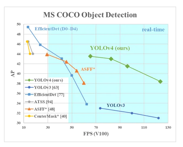
Yolov4 state-of-the-art detector which is faster (FPS)and more accurate (MS COCO AP[50…95] and AP50) than all available alternative real time detectors.
The original concept of one-stage anchor-based detectors has proven its viability. We have verified a large number of features, and selected for use such of them for improving the accuracy of both the classifier and the detector. [1]
Here ends the final part of this series. I know, it was a long journey, but I hope you now have a good grip in terms of the algorithmic perspective of YOLOv4.
Please check out other parts of our entire series on Yolov4 on our page VisionWizard.
It looks like you have a real interest in quality research work if you have reached till here. If you like our content and want more of it, please follow our page VisionWizard.
Do clap if you have learned something interesting and useful. It would motivate us to curate more quality content for you guys.
Thanks for your time :).
6. References
[1] YOLOv4
7. Connections
What this read builds on, and what builds on it. Hover a box for a preview.
Related
- Read · this builds on it
- Read · same topic: yolo, object detection; cites the same paper
- Read · closely linked
- Read · same topic: object detection
- Read · same topic: object detection
- Read · same topic: object detection
Go deeper
-
Start withRead
-
Read
-
Read
-
You are hereYOLOv4 — Version 4: Final VerdictRead